

Mechanical vibration is the oscillatory motion of a body or structure about a position of equilibrium, and this guide gives you the tools to model it, measure it, and control it. By the end, you will be able to:
- Set up and solve the equations of motion for single-degree-of-freedom (SDOF), multi-degree-of-freedom (MDOF), and continuous systems.
- Apply damping models, frequency response functions, and modal analysis to real engineering problems.
- Select appropriate sensors, configure a data-acquisition chain, and interpret FFT spectra.
- Choose between passive isolation, tuned absorbers, and active control strategies.
- Run a worked SDOF example in MATLAB and validate a finite-element model against an analytic solution.
Start with the worked SDOF example in Section 11 if you want an immediate hands-on check, then return to the theory sections to build the underlying intuition.
Principais conclusões
Mechanical vibration analysis follows a clear progression from SDOF analytic models through MDOF modal decomposition to FEM-based numerical simulation, with experimental validation at every stage.
| Ponto | Detalhes |
|---|---|
| SDOF is the foundation | Every vibration problem reduces to SDOF intuition: natural frequency, damping ratio, and frequency ratio govern the response. |
| Resonance occurs at r = 1 | When excitation frequency equals natural frequency, amplitude peaks; keep r below 0.7 or above 1.41 for safe operation. |
| Measure damping experimentally | Use the logarithmic decrement on a free-decay record; typical engineering ζ ranges from 0.01 for welded steel to 0.15 for rubber. |
| Validate FEM against analytic solutions | Confirm FEM natural frequencies match analytic values within 2–3% before adding model complexity. |
| WBV resonance is near 4–5 Hz | The human spine resonates at roughly 4–5 Hz; occupational exposure near this range is linked to low-back pain risk. |
Índice
- What is mechanical vibration, and what are its key parameters?
- How does the SDOF spring–mass–damper model work?
- How does forced vibration lead to resonance?
- Which damping models matter, and how do you measure damping?
- How do MDOF systems and modal analysis work?
- What happens in continuous systems: beams, rods, and plates?
- How do you measure vibrations correctly in practice?
- What are the main vibration isolation and control strategies?
- Which numerical tools and FEM workflows should you use?
- Worked SDOF example: set up, solve, and interpret
- What does research say about whole-body vibration risks?
- Where should you learn next? Courses, textbooks, and Portuguese resources
- How do energy methods and Lagrangian formulation apply to vibration?
- What are the implications of nonlinear vibration phenomena?
- How do you conduct modal testing and validate your model?
- What signal processing techniques go beyond FFT for vibration data?
- Building real intuition for vibration analysis: a practitioner’s view
- From vibration analysis to maintenance action: how Fullyops supports the workflow
- Sources
- FAQ
What is mechanical vibration, and what are its key parameters?
Mechanical vibration describes any oscillation of a mechanical system about a static equilibrium position. The motion can be periodic, random, or transient, and it arises whenever stored elastic energy converts repeatedly into kinetic energy and back again. Understanding the vocabulary is the first step to setting up any analysis correctly.
Primary kinematic variables:
- Displacement x (metres): the instantaneous position relative to equilibrium.
- Velocity ẋ (m s⁻¹): the first time derivative of displacement.
- Acceleration ẍ (m s⁻²): the second time derivative; the quantity most accelerometers measure directly.
- Amplitude X (metres): the peak value of displacement in a periodic signal.
- Period T (seconds): the time for one complete oscillation cycle.
- Frequência f (Hz): the number of cycles per second, related to period by f = 1/T.
- Angular frequency ω (rad s⁻¹): ω = 2πf, the form that appears naturally in differential equations.
- Natural frequency ωₙ (rad s⁻¹): the frequency at which an undamped system oscillates freely; for a simple spring–mass system, ωₙ = √(k/m).
- Transmissibility TR: the ratio of output amplitude (at a receiver) to input amplitude (at the source); values above 1 indicate amplification, values below 1 indicate isolation.
Standard notation throughout this guide uses x, ẋ, e ẍ for scalar SDOF motion, and bold x, ẋ, ẍ for MDOF vectors. The open-source textbook Vibration Mechanics follows the same convention and is a reliable reference for checking any derivation.
How does the SDOF spring–mass–damper model work?
The single-degree-of-freedom model is the foundation of all vibration analysis. Apply Newton’s second law to a mass m on a spring of stiffness k and a viscous dashpot of coefficient c, and the equation of motion for free vibration follows directly:
Dividing through by m and introducing ωₙ = √(k/m) and the damping ratio ζ = c / (2mωₙ) gives the standard normalised form:
O MIT OpenCourseWare engineering dynamics materials treat this derivation as the central pillar of undergraduate vibration teaching, and for good reason: every more complex model reduces to it under appropriate assumptions.
Energy viewpoint: in simple harmonic motion (SHM) with no damping, kinetic energy T = ½mẋ² and potential energy V = ½kx² are continuously exchanged. Their sum remains constant, which is why an undamped system oscillates indefinitely. Damping dissipates energy each cycle, reducing amplitude over time.
Damping cases and their analytic solutions
Concise free-vibration example: A steel bracket has m = 2 kg, k = 8,000 N m⁻¹, and c = 20 N s m⁻¹.
- ωₙ = √(8,000/2) = 63.25 rad s⁻¹ → fₙ = 10.07 Hz
- c_cr = 2 × 2 × 63.25 = 253 N s m⁻¹
- ζ = 20/253 = 0.079 (lightly underdamped)
- Damped natural frequency: ωd = 63.25 × √(1 − 0.079²) ≈ 63.05 rad s⁻¹
The response decays as x(t) = X e^(−5.0t) cos(63.05t + φ), where the initial conditions fix X and φ.
How does forced vibration lead to resonance?
When a harmonic force F(t) = F₀ sin(Ωt) is applied to an SDOF system, the steady-state displacement amplitude is:
X = (F₀/k) / √[(1 − r²)² + (2ζr)²]
where r = Ω/ωₙ is the frequency ratio. This expression is the magnitude of the frequency response function (FRF), and it contains everything you need to understand resonance and isolation.
Em r = 1 (excitation frequency equals natural frequency), the denominator reaches its minimum and amplitude peaks. For light damping, the peak amplitude approaches F₀ / (2ζk), which can be many times the static deflection. This is resonance, and it is the primary failure mode engineers must design around.
Practical rules for avoiding resonance and achieving isolation:
- Keep the operating frequency ratio r well below 0.7 or above √2 (≈1.41). Between these limits, transmissibility exceeds 1 regardless of damping.
- For isolation (transmissibility < 1), choose an isolator with ωₙ much lower than the excitation frequency, so r >> 1.
- For structures that must pass through resonance during run-up (turbines, motors), increase damping to limit peak amplitude and traverse the resonance quickly.
- Bandwidth (half-power bandwidth) is Δω ≈ 2ζωₙ; wider bandwidth means more energy dissipation but also a broader frequency range of elevated response.
- Never size a mounting system so that its natural frequency coincides with a dominant machine harmonic.
Which damping models matter, and how do you measure damping?
Viscous damping assumes the damping force is proportional to velocity: F_d = cẋ. This model is mathematically convenient and physically reasonable for fluid-film bearings and dashpots. The critical damping coefficient is c_cr = 2mωₙ, and the damping ratio ζ = c/c_cr is the single most useful non-dimensional parameter in vibration analysis.
Hysteretic (structural) damping models energy loss as proportional to displacement amplitude rather than velocity. It is expressed as a complex stiffness k(1 + iη), where η is the loss factor. Hysteretic damping is more realistic for welded or bolted structures under cyclic loading, but it is frequency-independent, which complicates time-domain simulation.
Measuring damping experimentally — logarithmic decrement method:
Record a free-decay time history and identify successive peak amplitudes x₁ e x_n separated by n cycles. The logarithmic decrement is:
δ = (1/n) ln(x₁/x_n)
Then ζ ≈ δ / (2π) for small damping. The MIT OCW materials demonstrate this procedure with physical pendulum and beam experiments, making it straightforward to replicate in a lab.
Typical engineering ζ ranges:
- Welded steel structures: 0.01–0.02
- Bolted or riveted steel: 0.02–0.05
- Reinforced concrete: 0.04–0.07
- Rubber isolators: 0.05–0.15
- Lightly damped precision instruments: < 0.005
Dica profissional: If your measured ζ is below 0.01, small errors in peak-picking dominate the logarithmic decrement calculation. Use at least 10 cycles of decay and average over multiple estimates to reduce uncertainty.
In the frequency domain, damping controls the sharpness of FRF peaks. A very low ζ produces a narrow, tall resonance peak that is easy to identify but sensitive to small frequency shifts — a useful diagnostic signal for detecting structural changes over time.
How do MDOF systems and modal analysis work?
Real structures have many degrees of freedom. The matrix equation of motion for an n-DOF system is:
M ẍ + C ẋ + K x = F(t)
where M, C, e K are the n × n mass, damping, and stiffness matrices, x is the displacement vector, and F is the forcing vector. For undamped free vibration (C = 0, F = 0), assuming harmonic motion x = φ e^(iωt) leads to the eigenvalue problem:
(K − ω² M) φ = 0
O n eigenvalues ωᵣ² give the natural frequencies, and the corresponding eigenvectors φ_r are the mode shapes. The Cambridge textbook Vibration of Mechanical Systems presents this derivation clearly alongside worked two-DOF examples that are ideal for building intuition before moving to numerical tools.
Modal superposition transforms the coupled physical equations into n independent SDOF equations in modal coordinates q_r, each governed by its own modal mass, stiffness, and damping. This decoupling is exact for undamped systems and approximate (modal damping assumption) for damped ones.
| System type | DOF | Analysis method | Typical application |
|---|---|---|---|
| SDOF | 1 | Analytic / closed-form | Preliminary design, isolator sizing |
| MDOF (few DOF) | 2–10 | Eigenvalue solver, modal superposition | Frames, coupled substructures |
| MDOF (large) | > 10 | FEM + modal truncation | Full structures, rotating machinery |
| Continuous | ∞ | Partial differential equations, FEM | Beams, plates, shells |
Modal truncation retains only the first m modes (m << n), which is valid when higher modes contribute negligibly to the response at the frequencies of interest. Truncation errors grow if the excitation contains significant energy near the truncated modes.
Common MDOF sources in practice:
- Multi-storey building frames under seismic or wind loading.
- Rotating machinery with coupled shaft, bearing, and casing dynamics.
- Vehicle suspensions with coupled body, axle, and tyre modes.
- Coupled substructures assembled from independently tested components.
What happens in continuous systems: beams, rods, and plates?
Continuous systems have distributed mass and stiffness, so their equations of motion are partial differential equations (PDEs) with, in principle, infinitely many natural frequencies.
The Euler–Bernoulli beam equation for transverse vibration is:
EI ∂⁴w/∂x⁴ + ρA ∂²w/∂t² = 0
where E is Young’s modulus, I the second moment of area, ρ the density, and A the cross-sectional area. Assuming harmonic motion and applying boundary conditions yields a characteristic equation whose roots give the mode frequencies.
For a cantilever beam of length L, the first natural frequency is approximately:
f₁ ≈ (1.875)² / (2π) × √(EI / ρAL⁴)
This formula shows the key scaling: f₁ increases with stiffness (EI) and decreases with mass per unit length (ρA) and the square of length. Doubling the length reduces f₁ by a factor of four.
Travelling waves versus standing modes:
- Travelling waves propagate energy along the structure and are the appropriate model for wave transmission, noise radiation, and shock propagation in long or semi-infinite structures.
- Standing modes arise from wave reflection at boundaries and are the appropriate model for resonance, modal testing, and structural dynamics of finite components.
For most engineering design problems involving resonance avoidance or isolation, the standing-mode (modal) viewpoint is the one to use. Travelling-wave models become important in acoustics, railway track dynamics, and pipeline vibration.
How do you measure vibrations correctly in practice?
Measurement quality determines whether your analysis is trustworthy. Poor sensor mounting and noisy baselines are among the most common sources of false-positive vibration diagnostics, so the checklist below deserves careful attention.
Sensor selection:
- Piezoelectric accelerometers — the standard choice for most industrial and structural measurements; wide frequency range (typically 0.5 Hz to several kHz), robust, and available in IEPE (ICP) and charge-output variants.
- Velocity sensors (geophones) — suited to low-frequency measurements (below ~10 Hz) where accelerometers lose sensitivity.
- Eddy-current displacement transducers — non-contact, ideal for shaft orbit measurements in rotating machinery where proximity to the surface is constant.
- MEMS accelerometers — low cost, suitable for IoT-based industrial vibration monitoring where high precision is not required.
Data-acquisition checklist:
- Set the sampling rate to at least 2.5 times the highest frequency of interest (Nyquist criterion); in practice, use 5–10 times to avoid aliasing artefacts.
- Apply an analogue anti-aliasing filter before the ADC, with a cut-off below half the sampling rate.
- Synchronise all channels to a common clock when measuring multiple points simultaneously.
- Record at least 10–20 averages for spectral estimates to reduce random noise.
- Log the sensor sensitivity, mounting method, and cable routing in the test record.
Signal processing steps:
- Detrend the time signal to remove DC offset and slow drift before computing spectra.
- Apply a window function (Hann is the default for general use; flat-top for amplitude accuracy) to reduce spectral leakage.
- Compute the FFT and examine the power spectral density (PSD) or FRF for peaks.
- Average multiple FFT blocks (Welch method) to reduce variance in the spectral estimate.
- Identify peaks and compare their frequencies against predicted natural frequencies from your analytic or FEM model.
SimScale’s vibration analysis overview describes this measurement-to-FRF workflow clearly and is a useful companion when setting up a first test campaign.
Interpreting an FFT peak: if a dominant peak appears at 47 Hz in your spectrum and your SDOF model predicts fₙ = 10.07 Hz, you are not seeing the fundamental mode. Check for higher harmonics of a rotating component (e.g. 47 Hz = blade-pass frequency of a 4-blade fan at 705 RPM) before concluding the model is wrong.
What are the main vibration isolation and control strategies?
The goal of vibration control is either to prevent vibration from reaching a sensitive receiver (isolation) or to reduce vibration at its source. The right strategy depends on the frequency range, the required attenuation, and the acceptable complexity.
Passive isolation uses springs, elastomeric pads, or wire-rope mounts to interpose a compliant element between source and receiver. The design rule is straightforward: choose an isolator with a natural frequency fᵢ such that r = f_excitation/fᵢ >> √2, which places the system well into the isolation region where transmissibility falls below 1. Rubber anti-vibration mounts, air springs, and coil springs are the most common hardware choices.
Tuned mass absorbers (TMAs) attach a secondary mass–spring system to the primary structure, tuned so that its natural frequency coincides with the excitation frequency. At that frequency, the absorber draws energy from the primary structure and reduces its amplitude substantially. TMAs are widely used in tall buildings (e.g. tuned mass dampers in skyscrapers) and in precision machine tools. Their limitation is narrow effective bandwidth: detune the excitation slightly and the benefit diminishes.

Active vibration control (AVC) uses sensors to measure vibration, a controller to compute a corrective signal, and actuators (piezoelectric, electromagnetic, or hydraulic) to apply a counter-force. AVC can achieve broadband attenuation and adapt to changing conditions, but it requires power, introduces stability risks, and demands careful controller design (typically PID, LQR, or H∞ methods).
Where each strategy applies:
- Passive isolation: machine foundations, precision optical tables, HVAC equipment, automotive engine mounts.
- Tuned absorbers: structures with a dominant single excitation frequency (fans, compressors, pedestrian bridges).
- Active control: aerospace structures, precision manufacturing, active noise and vibration cancellation in vehicles.
Control trade-offs to keep in mind:
- Passive systems are reliable and maintenance-free but fixed in their performance envelope.
- Active systems offer adaptability but add complexity, power consumption, and potential failure modes.
- Hybrid systems (passive + active) are increasingly common in high-performance applications where passive isolation handles broadband attenuation and active control handles residual narrowband disturbances.
Linking vibration findings to passos de manutenção preventiva is the practical bridge between analysis and action: once you know which frequency is causing wear, you can schedule isolator inspections and replacements before failure occurs.
Which numerical tools and FEM workflows should you use?
Numerical methods extend analytic solutions to geometries and boundary conditions that closed-form equations cannot handle. A structured workflow prevents the most common errors.
Step-by-step FEM workflow for vibration problems:
- Geometry and simplification: import or build the CAD model; suppress features smaller than 1/6 of the shortest wavelength of interest.
- Material properties: assign density, Young’s modulus, and Poisson’s ratio; verify units are consistent.
- Mesh: use at least 6 elements per wavelength for the highest mode of interest; refine at stress concentrations and joints.
- Boundary conditions: apply constraints carefully — over-constraining artificially raises natural frequencies.
- Modal analysis: extract the first m natural frequencies and mode shapes; compare the lowest modes against analytic estimates.
- Harmonic (frequency response) analysis: apply the forcing and sweep the frequency range; extract FRFs at points of interest.
- Post-processing: plot mode shapes, identify high-stress regions at resonance, and check transmissibility.
Tool selection:
- MATLAB / Simulink: the standard environment for prototyping SDOF and MDOF models, computing FRFs, and running parameter studies. An IOP conference study on MATLAB-based vibration research demonstrates how MATLAB accelerates both academic and industrial vibration analysis workflows.
- ANSYS: industry-standard FEM solver with dedicated structural dynamics and harmonic analysis modules; best for large, complex industrial models.
- COMSOL Multiphysics: strong for coupled physics problems (vibro-acoustics, piezoelectric transducers, fluid–structure interaction).
- Abaqus: preferred in aerospace and automotive sectors for nonlinear dynamics, contact, and composite structures.
Dica profissional: Before trusting any FEM result, validate the model against the analytic SDOF or Euler–Bernoulli beam solution for a simplified version of your geometry. If it does not, fix the model before adding complexity.
Worked SDOF example: set up, solve, and interpret
This example uses the bracket from Section 3 with an added harmonic force, so you can reproduce it directly in MATLAB.
Problem statement: m = 2 kg, k = 8,000 N m⁻¹, c = 20 N s m⁻¹, F₀ = 50 N, excitation frequency Ω = 50 rad s⁻¹.
Step-by-step analytic solution:
- ωₙ = √(8,000/2) = 63.25 rad s⁻¹; fₙ = 10.07 Hz.
- ζ = 20 / (2 × 2 × 63.25) = 0.079.
- Frequency ratio: r = 50/63.25 = 0.791.
- Static deflection: X_st = F₀/k = 50/8,000 = 6.25 × 10⁻³ m.
- Dynamic amplification factor: D = 1 / √[(1 − 0.791²)² + (2 × 0.079 × 0.791)²] = 1 / √[(0.375)² + (0.125)²] ≈ 1 / √(0.1406 + 0.0156) ≈ 1 / 0.395 ≈ 2.53.
- Steady-state amplitude: X = 6.25 × 10⁻³ × 2.53 ≈ 15.8 × 10⁻³ m (15.8 mm).
MATLAB pseudocode:
m = 2; k = 8000; c = 20; F0 = 50;
wn = sqrt(k/m);
zeta = c / (2*m*wn);
Omega = linspace(0, 2*wn, 500);
r = Omega / wn;
D = 1 ./ sqrt((1 - r.^2).^2 + (2*zeta*r).^2);
X = (F0/k) * D;
plot(Omega/(2*pi), X*1000)
xlabel('Frequency (Hz)'); ylabel('Amplitude (mm)')
Interpreting the results:
- The peak amplitude occurs near fₙ = 10.07 Hz, not at the operating frequency of 7.96 Hz (Ω = 50 rad s⁻¹). The operating point sits at r = 0.79, below resonance.
- The safety margin to resonance is approximately 21% in frequency ratio. For a safety-critical component, this may be insufficient; consider stiffening the bracket to raise fₙ above 15 Hz.
- If you move to a FEM model of the same bracket, run a mesh sensitivity check: halve the element size and confirm that fₙ changes by less than 2%.
What does research say about whole-body vibration risks?
Whole-body vibration (WBV) is a specific and practically important subset of the effects of mechanical vibration, relevant to vehicle operators, construction workers, and anyone seated on vibrating machinery for extended periods.
A peer-reviewed review published on PMC reports that the resonant frequency of the human spine occurs in the low-frequency range relevant to vibration exposure, and occupational exposure near these frequencies is associated with increased risk of low-back pain and spinal tissue changes. The review also notes that precise dose–response quantification remains an open research question, so engineers should treat WBV limits as precautionary thresholds rather than exact safety boundaries.
Key finding: The human spine resonates at roughly 4–5 Hz. Prolonged occupational vibration near this range is linked to elevated low-back pain risk and spinal tissue changes, though the precise dose–response relationship is still being quantified.
It is worth distinguishing occupational WBV from therapeutic whole-body vibration exercise (WBVE). Research published via Frontiers indicates that controlled WBVE protocols, especially variable-frequency and side-alternating types, may have therapeutic benefits depending on frequency, amplitude, and application mode, which influence whether vibration is harmful or beneficial.
Measurement checklist for occupational WBV monitoring:
- Measure frequency content across the 0.5–80 Hz band, with particular attention to the 4–8 Hz range.
- Record vibration magnitude in all three axes (vertical z, fore-aft x, lateral y) using a seat-pad accelerometer.
- Log exposure duration and calculate daily vibration dose value (VDV) or root-mean-square (RMS) acceleration per ISO 2631-1.
- Document operating conditions (vehicle speed, surface type, load) alongside the vibration data.
- Repeat measurements periodically to track changes in equipment condition.
Involve an occupational health specialist for medical interpretation of exposure data. Engineers can measure and quantify; clinical assessment of individual health risk requires qualified medical input.
Where should you learn next? Courses, textbooks, and Portuguese resources
A structured study plan moves from analytic foundations to numerical tools to experimental validation. The resources below are ordered to support that progression.
Online courses:
- Coursera’s Mechanical Vibration course combines modular video lectures with MATLAB exercises and worked examples. It is the most accessible starting point for students who want both theoretical grounding and computational practice in one place.
- MIT OpenCourseWare Engineering Dynamics (2.003SC) provides full lecture notes, problem sets, and demonstration videos at no cost. The damping estimation and modal analysis modules are particularly strong for building physical intuition.
Textbooks (in recommended reading order):
- Vibration Mechanics (open-source, University of South Carolina) — start here for concise SDOF derivations and energy explanations with undergraduate worked examples.
- Vibration of Mechanical Systems (Cambridge University Press) — follow with this for MDOF formulations and an introduction to FEM links; compact enough to read alongside a course.
- Benaroya, Han, and Nagurka, Mechanical Vibration: Analysis, Uncertainties, and Control — use this for deeper coverage of random vibration, control, and uncertainty quantification.
- Ewins, Modal Testing: Theory, Practice and Application — the standard reference once you move to experimental work.
Software documentation:
- MATLAB documentation (MathWorks): the Signal Processing Toolbox and Structural Dynamics examples are the most relevant starting points.
- ANSYS Help: the Mechanical APDL Structural Analysis Guide covers modal and harmonic analysis setup in detail.
- COMSOL Multiphysics: the Structural Mechanics Module user guide includes vibration tutorials with step-by-step FEM setups.
- Abaqus documentation: the Analysis User’s Guide sections on frequency extraction and steady-state dynamics are the key references.
Finding resources in Portugal: Portuguese universities with strong mechanical engineering programmes, including Instituto Superior Técnico (IST) in Lisbon and the University of Porto’s Faculty of Engineering (FEUP), maintain laboratory facilities for vibration testing and offer postgraduate modules in structural dynamics. Check their open-access repositories (Repositório Científico de Acesso Aberto de Portugal, RCAAP) for theses and datasets. The Ordem dos Engenheiros also lists accredited continuing professional development courses in dynamics and maintenance engineering.
How do energy methods and Lagrangian formulation apply to vibration?
Newton’s second law works well for simple geometries, but for systems with constraints, multiple coordinates, or complex kinematics, the Lagrangian approach is more systematic and less error-prone.
The Lagrangian L = T − V (kinetic energy minus potential energy) leads to Lagrange’s equations:
d/dt (∂L/∂q̇ᵢ) − ∂L/∂qᵢ = Qᵢ
where qᵢ are generalised coordinates and Qᵢ are generalised non-conservative forces (including damping). For a conservative SDOF system with T = ½mẋ² and V = ½kx², Lagrange’s equation reproduces the familiar mẍ + kx = 0 directly, confirming consistency with Newton’s approach.
The real power appears in MDOF systems. For a two-DOF system with coordinates q₁ e q₂, writing T e V in terms of both coordinates and applying Lagrange’s equations automatically generates the coupled matrix EOM without needing to draw free-body diagrams for each mass separately. This is particularly valuable for systems with geometric constraints, such as pendulums, linkages, or rotating frames.
Rayleigh’s method offers a quick estimate of the fundamental natural frequency without solving the full eigenvalue problem. By assuming a trial mode shape and equating maximum kinetic and potential energies, you obtain:
The estimate is always an upper bound for the true fundamental frequency, and it converges rapidly when the trial shape resembles the actual first mode. Engineers use it for quick sanity checks before running a full FEM modal analysis.
What are the implications of nonlinear vibration phenomena?
Linear vibration theory assumes small displacements, linear material behaviour, and time-invariant parameters. Real industrial assets frequently violate at least one of these assumptions, and the consequences can be significant.
Key nonlinear phenomena:
- Amplitude-dependent natural frequency: in a hardening spring (e.g. a coil spring approaching its solid height), the effective stiffness increases with amplitude, so the resonance frequency shifts upward as amplitude grows. A softening spring shows the opposite. Neither behaviour is captured by a linear model.
- Jump phenomena: when a nonlinear system is swept through resonance, the response amplitude can jump discontinuously at a critical frequency, then follow a different path on the return sweep. This hysteresis in the frequency response is a diagnostic indicator of nonlinearity.
- Subharmonic and superharmonic resonances: a nonlinear system can resonate at fractions or multiples of the excitation frequency, producing peaks in the spectrum at Ω/2, Ω/3, or 2Ω, 3Ω. These are absent in linear models and can be mistaken for structural damage or measurement artefacts.
- Chaos: strongly nonlinear systems under periodic forcing can exhibit aperiodic, sensitive-to-initial-conditions behaviour. Duffing’s oscillator is the canonical example studied in undergraduate nonlinear dynamics.
In practice, the Vibration Mechanics open textbook recommends starting with equivalent linearisation: replace the nonlinear stiffness or damping with a linear equivalent that matches the energy dissipated or stored at the operating amplitude. This gives a first approximation that is often sufficient for preliminary design, while flagging cases where a full nonlinear analysis in MATLAB or Abaqus is warranted.
How do you conduct modal testing and validate your model?
Modal testing is the experimental counterpart to numerical modal analysis. Its output — a set of measured natural frequencies, damping ratios, and mode shapes — serves two purposes: characterising an unknown structure and validating a FEM model.
Standard experimental modal analysis (EMA) procedure:
- Excitation: use an instrumented impact hammer (for broadband, low-energy excitation) or an electrodynamic shaker with a swept-sine or random signal (for higher force levels or controlled frequency content).
- Response measurement: place accelerometers at a grid of points covering the structure; the grid density determines which modes can be resolved spatially.
- FRF measurement: compute the FRF between each response point and the excitation point using a dual-channel FFT analyser or equivalent software (e.g. MATLAB’s
tfestimatefunction). - Curve fitting: fit analytic FRF expressions to the measured data using a modal parameter extraction algorithm (e.g. peak-picking, circle-fit, or polyreference least-squares methods). Software such as ME’scope or LMS Test.Lab automates this step.
- Mode shape assembly: collect the residues from each FRF to assemble the full mode shape vector for each identified mode.
Model validation criteria:
- Natural frequency agreement within 5% between FEM and test for the first several modes is a common acceptance criterion in structural dynamics.
- The Modal Assurance Criterion (MAC) quantifies mode shape correlation: MAC = 1 indicates perfect agreement, MAC < 0.9 suggests significant discrepancy requiring model updating.
- Damping ratios from FEM (often assumed modal) should be compared with measured values; large discrepancies indicate that the damping model needs revision.
Model updating adjusts FEM parameters (material properties, joint stiffnesses, boundary conditions) to minimise the difference between predicted and measured modal properties. This is an active research area, and tools such as MATLAB’s Optimization Toolbox or dedicated FEM updating packages support it.
What signal processing techniques go beyond FFT for vibration data?
The FFT is the workhorse of vibration signal processing, but it assumes stationarity: the statistical properties of the signal do not change over time. Many real vibration signals, particularly those from rotating machinery with varying speed or from structures undergoing transient events, are non-stationary. Several techniques address this limitation.
Wavelet analysis decomposes a signal into time-frequency atoms of variable duration, using short windows at high frequencies and long windows at low frequencies. This multi-resolution property makes wavelets well suited to detecting transient events (impacts, crack propagation, bearing defects) that appear briefly in the signal. The continuous wavelet transform (CWT) and discrete wavelet transform (DWT) are both available in MATLAB’s Wavelet Toolbox.
Short-time Fourier transform (STFT) applies a sliding FFT window to produce a spectrogram: a time-frequency map showing how spectral content evolves. The trade-off between time resolution and frequency resolution is fixed by the window length, which is the key limitation compared with wavelets.
Hilbert–Huang transform (HHT) combines empirical mode decomposition (EMD) with the Hilbert transform to extract instantaneous frequency and amplitude from non-stationary, nonlinear signals. It requires no predefined basis functions, making it data-adaptive, though it is computationally intensive and sensitive to noise.
Order tracking is specific to rotating machinery: it resamples the vibration signal from the time domain to the angular domain (using a tachometer reference), so that spectral peaks appear at integer multiples of shaft rotation speed rather than at fixed Hz values. This eliminates smearing caused by speed variation and makes it straightforward to identify bearing defect frequencies, gear mesh frequencies, and imbalance harmonics.
For industrial vibration monitoring, combining FFT-based baseline trending with wavelet-based transient detection gives a practical and computationally manageable approach. MATLAB’s Signal Processing Toolbox and Wavelet Toolbox together cover all four techniques described above.
Building real intuition for vibration analysis: a practitioner’s view
The gap between understanding vibration theory and being able to use it confidently in practice is wider than most courses acknowledge. Textbooks present clean derivations; real structures present noisy data, uncertain boundary conditions, and nonlinearities that do not announce themselves.
The most effective learning path is not to read more theory but to close the loop between model and measurement as quickly as possible. Build an SDOF model in MATLAB, measure the free decay of a simple beam or spring-mass rig, extract ζ using the logarithmic decrement, and compare it with your model’s prediction. That single exercise teaches more about damping than three lectures on viscous versus hysteretic models, because you encounter the real sources of error: sensor noise, imperfect initial conditions, and the sensitivity of peak-picking to signal length.
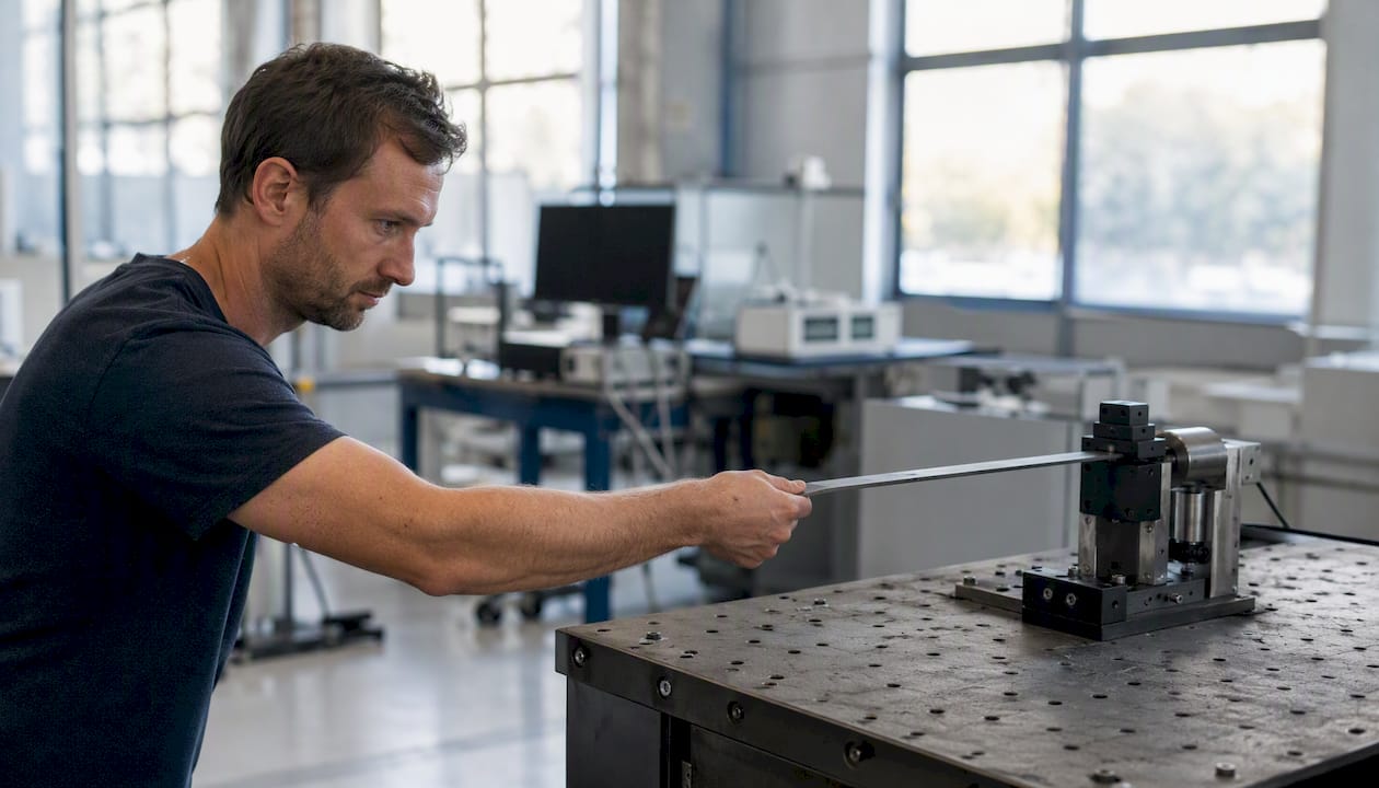
Keep a validation notebook. For every FEM model you build, record the analytic check you ran before trusting the result, the mesh sensitivity result, and the measured natural frequency if you have one. Over time, this notebook becomes a personal database of modelling decisions and their consequences, which is exactly the kind of accumulated judgement that separates a competent analyst from a capable one.
One habit that accelerates progress significantly: reproduce a classic experiment from the literature. Reproducing Benaroya’s two-DOF pendulum experiment, or the cantilever beam modal test from MIT OCW, forces you to confront every step of the measurement chain rather than accepting published results passively. Small experimental notes, even unpublished ones shared within a research group, build the documentation habit that industrial vibration monitoring demands.
The tools matter less than the workflow. Whether you use MATLAB, ANSYS, or COMSOL, the discipline of analytic check → numerical model → experimental validation → model update is what produces reliable results. Engineers who skip the analytic check because “the FEM will handle it” are the ones who miss a factor-of-two error in boundary conditions and spend days debugging a model that was wrong from the first mesh.
From vibration analysis to maintenance action: how Fullyops supports the workflow
Identifying a vibration problem is only half the task. Converting that finding into a scheduled inspection, a corrective work order, and a documented history is where many industrial teams lose the value of their analysis.
Fullyops is a cloud-based asset and field service management platform designed for exactly this handoff. When vibration monitoring identifies a bearing approaching its wear threshold, Fullyops allows maintenance managers to raise a work order and track it to completion with full documentation of the measurement findings, the corrective action taken, and the technician’s time. The platform’s operations analytics module supports trend detection, so recurring vibration-related faults on the same asset become visible across work order history rather than remaining isolated incidents.
For industrial teams in Portugal managing rotating machinery, HVAC plant, or production equipment, Fullyops provides the operational layer that turns vibration data into maintenance software workflows with assigned technicians, spare-parts tracking, and compliance records. The result is a closed loop: measure, analyse, act, document, and repeat.
Sources
- Mechanical vibration | MIT OpenCourseWare
- Review of whole‑body vibration and spinal health (PMC)
- Vibration Mechanics (open textbook)
FAQ
What is mechanical vibration?
Mechanical vibration is the oscillatory motion of a body or structure about a position of static equilibrium, driven by the periodic exchange of kinetic and potential energy. It is characterised by natural frequency, amplitude, and damping ratio.
What are the main types of mechanical vibration?
The four principal types are free vibration (no external forcing after an initial disturbance), forced vibration (sustained by a continuous external force), damped vibration (energy is dissipated each cycle), and undamped vibration (no energy loss, perpetual oscillation). Systems can exhibit any combination of these characteristics simultaneously.
What is the mechanics of vibration?
The mechanics of vibration describes how forces, masses, and elastic elements interact to produce oscillatory motion, governed by Newton’s second law or Lagrange’s equations. For an SDOF system, the equation of motion mẍ + cẋ + kx = F(t) captures this interaction completely.
How many types of mechanical vibrations are there?
Vibration is commonly classified by four criteria: the presence or absence of external forcing (free vs. forced), the degree of energy dissipation (damped vs. undamped), the number of degrees of freedom (SDOF, MDOF, continuous), and the nature of the excitation (deterministic vs. random). These classifications overlap, so a real system might be described as “forced, underdamped, MDOF with random excitation.”
How do you reduce mechanical vibration in industrial equipment?
The most effective approach depends on the frequency ratio. For excitation well above the system’s natural frequency, passive isolation using springs or elastomeric mounts reduces transmissibility below 1. For a dominant single excitation frequency, a tuned mass absorber is highly effective. Active vibration control suits broadband or variable-frequency problems where passive methods are insufficient.
Recomendado
- Effects analysis in FMEA: practitioner guide for engineers – FullyOps
- Operation and maintenance: the complete UK guide for 2026
- Exemplos de manutenção preventiva para prolongar a vida útil de ativos