Vibration data for engineers: a practical guide

Vibration data is the time-series record of mechanical oscillation, measured as displacement, velocity, or acceleration, that engineers use to detect, diagnose, and trend faults in rotating and reciprocating machinery before those faults cause unplanned downtime. It is the primary input for condition monitoring and the foundation of any credible predictive maintenance programme.

Early fault detection: vibration monitoring systems can identify bearing wear, misalignment, and unbalance long before faults become audible or visible, reducing unplanned stoppages.
Required assets: a measurement chain of sensors, data acquisition hardware, and signal-processing software, governed by standards such as ISO 20816 and API 670.
Learning resources: public datasets (Case Western Reserve, NASA Prognostics, Zenodo VBL-VA001) and toolboxes such as the VibrationData Toolbox give engineers validated material to develop and test algorithms.

When a vibration alarm is confirmed, Fullyops converts that finding into a tracked work order, stores the measurement metadata against the asset record, and keeps the intervention visible to the whole maintenance team.

Principais conclusões

Vibration data delivers diagnostic value only when the full chain is correct: the right sensor, properly mounted, with clean acquisition, rigorous signal processing, and findings linked to tracked maintenance action.

Ponto	Detalhes
Match sensor to frequency range	Use piezo accelerometers for high-frequency bearing faults, velocity transducers for mid-band structural vibration, and proximity probes for shaft displacement.
Stud-mount for high-frequency work	Stud mounting preserves response up to approximately 15 kHz; adhesive and magnetic mounts reduce that ceiling significantly.
Apply Nyquist margin in practice	Sample at 2.5–4 times the highest frequency of interest and set anti-alias filter cut-off at or below 40% of the sampling rate.
Normalise features for speed and load	Raw vibration amplitudes vary with operating point; without normalisation, trend charts can misdirect maintenance priorities.
Use envelope analysis for bearings	Band-pass filter, rectify, and apply a second FFT to reveal bearing defect frequencies before overall RMS rises.
Fullyops links findings to action	Fullyops converts confirmed vibration diagnoses into tracked work orders with asset metadata, severity ranking, and intervention history.

For further reading and algorithm validation, the Zenodo VBL-VA001 dataset, the NASA Prognostics Data Repository, and the VibrationData Toolbox are the most practical starting points.

Índice

What does vibration data actually measure?
How mechanical motion becomes electrical signals: sensors and mounting
Displacement, velocity, or acceleration: which measure should you use?
DAQ fundamentals: how to set up data acquisition correctly
How to turn raw signals into diagnostic features
Common fault signatures and how to diagnose them
How to collect vibration data correctly in the field
Software, toolboxes, and learning resources for vibration analysis
Why vibration data only delivers value when it drives action
Fullyops helps you act on vibration findings, not just record them
Sources
FAQ

What does vibration data actually measure?

Vibration data records three physical quantities: displacement (how far a surface moves, in micrometres or mils), velocity (how fast it moves, in mm/s or in/s), and acceleration (how rapidly velocity changes, in m/s² or g). Each quantity emphasises a different part of the frequency spectrum, which is why the choice of measurement parameter is a diagnostic decision, not just a hardware one.

Engineers use this data for several distinct purposes:

Early fault detection: bearing raceway defects, gear-mesh anomalies, and developing misalignment all produce characteristic frequency patterns that appear in vibration spectra weeks or months before failure.
Severity trending: plotting overall vibration level over time reveals whether a machine is stable, gradually deteriorating, or accelerating towards failure.
Root-cause isolation: comparing amplitude, phase, and frequency content across measurement points separates mechanical sources (unbalance, looseness) from structural ones (resonance, foundation problems).
Acceptance testing: post-repair or post-installation vibration measurements confirm that a machine meets the severity limits defined in ISO 20816 before returning to service.

Typical applications span power-generation turbines, centrifugal pumps, reciprocating compressors, industrial gearboxes, and electric motors. A systematic review of vibration analysis applications confirms that combining trending, comparative, and signature analysis gives more accurate diagnostics than any single technique alone, a finding consistent across industries from petrochemical to wind energy.

For maintenance teams, the practical value of vibration monitoring is straightforward: it converts an invisible physical process into a quantified, time-stamped record that supports predictive maintenance decisions rather than calendar-based guesswork.

How mechanical motion becomes electrical signals: sensors and mounting

The measurement chain starts at the sensor. Choosing the wrong transducer, or mounting it incorrectly, corrupts every downstream step regardless of how sophisticated the analysis software is.

Sensor types and their roles

Piezoelectric accelerometers: the most common choice for industrial condition monitoring. They measure acceleration directly, cover a wide frequency range (typically 0.5 Hz to 15 kHz depending on model), and suit bearing-defect detection, gear-mesh analysis, and high-frequency structural response. Industry guidance maps piezo accelerometers specifically to high-frequency acceleration and early bearing-defect detection.
Eddy-current (proximity) probes: non-contact sensors that measure shaft displacement relative to a bearing housing. Used in API 670-compliant installations on large turbines, compressors, and pumps where shaft orbit and relative motion matter more than housing vibration.
Velocity transducers: electrodynamic sensors suited to mid-frequency structural vibration (typically 10 Hz to 1 kHz). Useful on slow-speed machinery where acceleration signals are weak but velocity amplitudes are still diagnostically meaningful.
Laser vibrometers: non-contact, high-precision instruments for surfaces that cannot be contacted (hot, rotating, or fragile). Primarily a laboratory and R&D tool rather than a routine field instrument.

Mounting best-practice checklist

Mounting method directly determines the usable frequency range of the measurement. Stud-mounted accelerometers preserve high-frequency response up to a high frequency; adhesive and magnetic mounts progressively reduce that ceiling.

Utilize stud mounting whenever the highest fault-frequency of interest exceeds 5 kHz (e.g., early-stage bearing defects at high shaft speeds).
Clean and degrease the mounting surface; surface roughness introduces resonance artefacts.
Apply a thin layer of coupling grease under magnetic or adhesive mounts to improve contact.
Route cables away from heat sources, sharp edges, and high-voltage conductors; use cable ties at regular intervals to prevent cable-induced noise.
Verify sensor grounding: floating or double-grounded sensors introduce 50/60 Hz electrical noise into the signal.
Seal connectors in wet or dusty environments with appropriate IP-rated boots.
Mark mounting locations permanently (paint pen or centre punch) to guarantee repeatability across measurement campaigns.

Dica profissional: Before a long-term monitoring campaign, perform a quick frequency-response check by tapping the sensor mount with a calibrated impulse hammer and comparing the resulting spectrum to the sensor’s published response curve. Any resonance peak inside your frequency band of interest means the mount needs to change.

The VibrationData Toolbox by Tom Irvine and the technical guidance published by DMC both provide worked examples and downloadable demonstrations that are particularly useful when verifying sensor and mounting configurations in the early stages of a monitoring programme.

Displacement, velocity, or acceleration: which measure should you use?

The answer depends on the frequency band where the fault energy sits and the severity metric your standard requires. Applying the wrong parameter leads to low signal-to-noise ratios and missed faults.

Measurement	Typical frequency band	Common fault targets
Displacement	Below 10 Hz	Shaft bow, slow-speed unbalance, journal bearing wear, rotor rub
Velocity	10 Hz to 1 kHz	Unbalance, misalignment, looseness, resonance, structural vibration
Acceleration	1 kHz to 20 kHz	Rolling-element bearing defects, gear-mesh harmonics, cavitation

A few practical rules that hold across most industrial applications:

ISO 20816 uses velocity (mm/s RMS) as the primary severity metric for most rotating machinery because it correlates well with the energy content of vibration across the mid-frequency band where most mechanical faults radiate.
API 670 specifies proximity probes for shaft displacement on large turbomachinery, where relative shaft motion inside the bearing is the critical parameter.
For early bearing-defect detection, acceleration (or its envelope) is the correct choice: defect-frequency energy sits at multiples of the bearing defect frequencies (BPFO, BPFI, BSF, FTF), which typically fall in the 1–20 kHz range.
On very slow-speed machinery (below 60 RPM), displacement is often the only parameter with sufficient amplitude to be measurable reliably.

Sensor technology guidance confirms this mapping: proximity probes for displacement and shaft motion, velocity transducers for mid-band structural vibration, and piezoelectric accelerometers for high-frequency acceleration.

DAQ fundamentals: how to set up data acquisition correctly

Clean data acquisition is where most field measurement errors originate. Incorrect sampling rates, missing anti-alias filters, and poor trigger configuration produce spectra that look plausible but contain aliased or truncated content.

Sampling-rate rules

The Nyquist theorem requires a sampling rate at least twice the highest frequency of interest. In practice, apply a margin of 2.5 to 4 times: if you need to resolve content up to 10 kHz, sample at 25–40 kHz. For envelope analysis of bearing defects, where the demodulated signal may contain content up to 20 kHz, sampling at 50–100 kHz is common. USGS technical guidance on real-time vibration analysis reinforces the importance of anti-alias filtering and appropriate sampling margins for field acquisition systems.

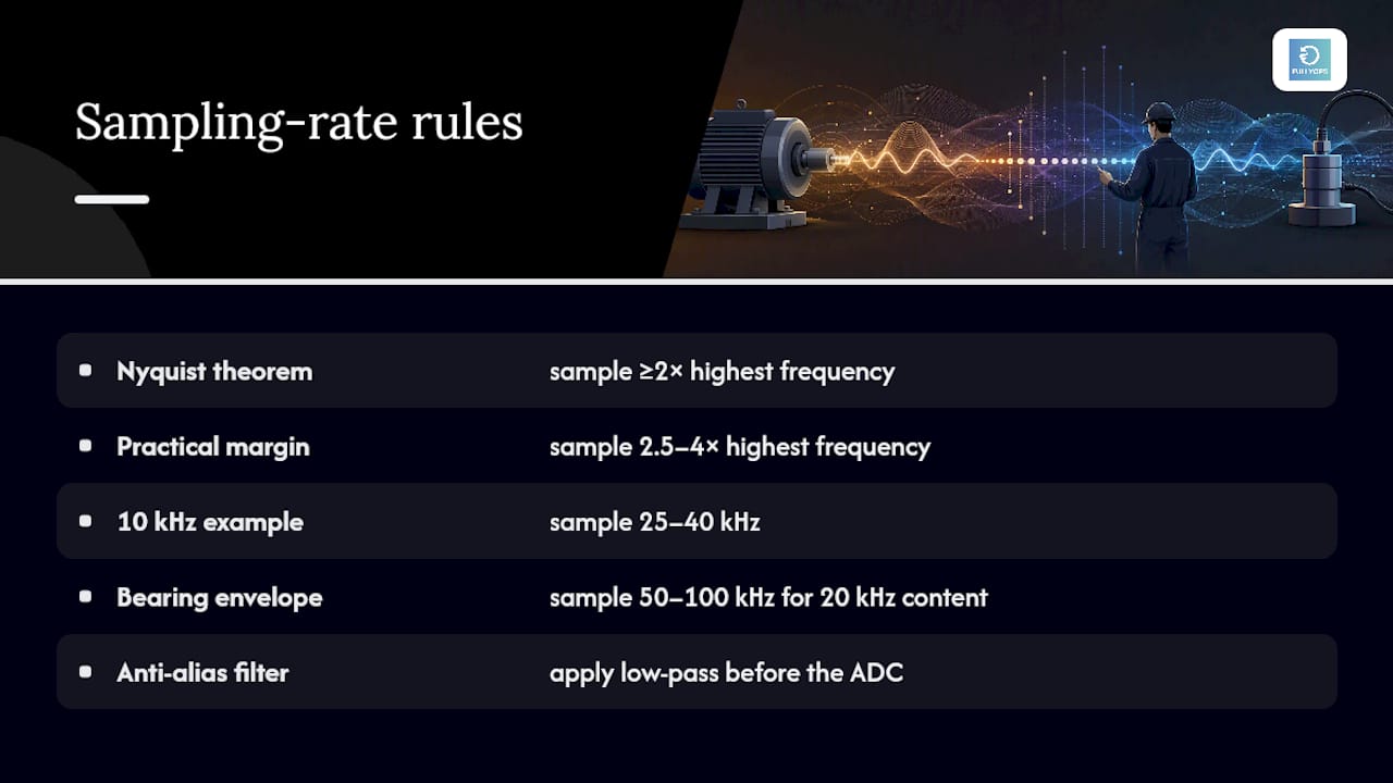
Anti-alias (low-pass) filters must be applied before the analogue-to-digital converter, not after.

DAQ setup checklist

Confirm sensor calibration certificate is current and the sensitivity value is entered correctly in the DAQ software.
Set IEPE (ICP) excitation current to the value specified by the sensor manufacturer (typically 2–10 mA).
Select the correct input range: too wide wastes resolution; too narrow causes clipping.
Configure anti-alias filter cut-off at or below 40% of the sampling rate.
Set trigger conditions: free-run for steady-state machines; external trigger or tachometer pulse for transient or order-tracked captures.
Synchronise channels when using multichannel acquisition: verify that all channels share the same clock and that inter-channel delay is within specification.
Verify cable integrity with a quick continuity check before starting a long campaign.

Single-channel vs multichannel and steady-state vs transient

Single-channel capture is adequate for routine trending on a single bearing location. Multichannel acquisition becomes necessary when you need phase relationships between measurement points (e.g., to distinguish unbalance from misalignment) or when you are building a labelled dataset for machine-learning validation.

Steady-state capture, where the machine runs at constant speed and load, produces the cleanest FFT spectra and is the standard approach for periodic route-based monitoring. Transient capture, recording run-up or coast-down, reveals resonance frequencies and critical speeds that are invisible in steady-state data. The systematic review confirms that combining steady-state and real-time multichannel approaches improves diagnostic accuracy.

How to turn raw signals into diagnostic features

Raw vibration signals are noisy and dense. The processing sequence below converts them into features that carry diagnostic meaning.

Processing sequence

Pre-process: remove DC offset (de-trend), check for clipping, and apply any necessary resampling or order-tracking to compensate for speed variation.
Band-pass filter: select the frequency band of interest before envelope analysis; this isolates fault-related energy from the background noise floor. Feature extraction research identifies band-pass filtering as the critical step that makes envelope analysis reliable.
Apply FFT: use a Hanning or flat-top window (Hanning for frequency resolution, flat-top for amplitude accuracy), select an appropriate block size (typically 1,024–16,384 samples), and average multiple blocks to reduce variance.
Envelope analysis: rectify and low-pass filter the band-passed signal, then apply a second FFT to the envelope to reveal bearing defect frequencies. Practical vibration analysis guidance recommends envelope demodulation as the most effective technique for rolling-element bearing diagnostics.
Cepstrum analysis: apply the inverse FFT of the log spectrum to identify families of equally spaced sidebands, particularly useful for gearbox modulation detection.
Order tracking: resample the signal with respect to shaft angle rather than time; this sharpens order-related peaks and is especially valuable for variable-speed machines. The MDPI Applied Sciences special issue highlights order tracking and STFT as repeatedly recommended methods for rotating machinery diagnostics.
Wavelet or STFT: apply when the signal is non-stationary (e.g., during run-up or under fluctuating load) and you need time-frequency resolution simultaneously.
Normalise features by operating variables: adjust extracted features for speed and load before trending (see Pro Tip below).

Diagnostic features and what they signal

RMS (overall): general severity indicator; rises as fault energy increases across the band.
Peak and crest factor: crest factor (peak/RMS) is sensitive to impulsive content; elevated crest factor often precedes a rise in RMS in early-stage bearing faults.
1X amplitude and phase: dominant at running speed; primary indicator of unbalance.
2X and axial 1X: elevated 2X with a strong axial component suggests misalignment.
Bearing defect frequencies (BPFO, BPFI, BSF, FTF): peaks at these frequencies in the envelope spectrum confirm rolling-element bearing damage.
Gear-mesh frequency and sidebands: amplitude modulation sidebands around gear-mesh frequency indicate tooth wear or load distribution problems.
Cepstral peaks (rahmonic): identify the pitch period of sideband families in gearbox signals.
Sub-synchronous content: frequencies below 1X can indicate oil-film instability (whirl/whip) in fluid-film bearings.

Dica profissional: Always normalise vibration features for speed and load before plotting trends. A bearing running at 3,000 RPM under full load produces higher raw vibration amplitudes than the same bearing at 1,500 RPM under half load. Without normalisation, a trend chart can show an apparent deterioration that is simply a change in operating point, misdirecting maintenance priorities. Vibration analysis research confirms that operating-context normalisation is one of the most commonly overlooked steps in industrial monitoring programmes.

Common fault signatures and how to diagnose them

Each mechanical fault leaves a characteristic pattern in the vibration spectrum. Recognising these patterns quickly is the core diagnostic skill.

Unbalance: dominant 1X peak at running speed, consistent phase, amplitude proportional to speed squared. Confirmed by phase measurement: a single-plane unbalance shows a stable phase angle at 1X.
Misalignment: elevated 2X (and sometimes 3X) with a strong axial vibration component at 1X and 2X. Angular misalignment tends to produce high axial 1X; parallel misalignment produces high radial 2X.
Rolling-element bearing defect: impulsive time waveform with elevated crest factor; envelope spectrum shows peaks at BPFO, BPFI, BSF, or FTF with harmonics. Early-stage faults appear in the envelope before any rise in overall RMS.
Mechanical looseness: multiple harmonics of running speed (3X, 4X, and beyond) with a noisy, irregular time waveform. Sub-harmonic content (0.5X) can appear with severe looseness.
Resonance: amplitude that peaks sharply at a specific frequency regardless of running speed, confirmed by a run-up or coast-down test where the peak tracks frequency rather than order.
Gear-mesh faults: peaks at gear-mesh frequency (number of teeth × shaft speed) with amplitude-modulated sidebands at shaft speed intervals. Increasing sideband amplitude relative to the mesh peak indicates developing tooth damage.

Diagnostic quick-check flow

When you spot an anomalous pattern, follow this sequence before concluding a diagnosis:

Confirm operating speed from a tachometer or nameplate; verify the machine is at its normal load point.
Check phase at 1X across multiple measurement points to distinguish unbalance (consistent phase) from looseness (erratic phase).
Compare amplitudes across radial and axial directions: axial dominance points to misalignment or thrust issues.
Apply speed and load normalisation to confirm the feature is fault-related, not operating-condition-related.
Trend the feature over time: a single elevated reading is less significant than a consistent upward trend.

Electrical-origin signatures

Broken rotor bars in induction motors produce sidebands around line frequency at intervals of twice the slip frequency. Electromagnetic forces from air-gap eccentricity generate peaks at twice line frequency (100 Hz in a 50 Hz system) and its harmonics. These differ from mechanical signatures because their frequency is tied to electrical supply frequency rather than shaft speed, and they do not shift with load in the same way mechanical faults do.

How to collect vibration data correctly in the field

A consistent, documented collection procedure is what separates a reliable monitoring programme from a collection of disconnected measurements.

Step-by-step collection checklist

Safety pre-check: confirm the machine is in its normal operating state, guards are in place, and you have a safe working position away from rotating parts.
Review the measurement plan: confirm the measurement points, axes (radial horizontal, radial vertical, axial), sensor type, and DAQ settings for this asset.
Inspect the mounting location: clean the surface, check for corrosion or damage, and verify the permanent location mark is intact.
Mount the sensor: apply the correct mounting method for the frequency range required; torque stud-mounted sensors to the manufacturer’s specification.
Connect and configure the DAQ: enter sensor sensitivity, set sampling rate, configure anti-alias filter, and select the correct input range.
Verify the signal: view the live time waveform before recording; confirm there is no clipping, no obvious electrical noise, and that the amplitude is in a sensible range for the machine type.
Capture steady-state data: record at least 10–20 averages for spectral analysis; longer for low-frequency content.
Capture transient data if required: for run-up or coast-down, arm the trigger and record through the speed range of interest.
Perform a quick sanity check: inspect the time waveform for clipping or dropout; view the FFT and confirm 1X and 2X peaks are present and at the expected frequencies.
Log anomalies: note any unusual observations (noise, temperature, visible leaks) in the measurement record.
Disconnect and store the sensor: protect connectors and cables from contamination.

File naming and metadata template

Every measurement file should carry the following metadata, either in the filename or in an accompanying log:

Asset ID and location code
Measurement point identifier and axis
Sensor ID and sensitivity value
Sampling rate and record length
Operating speed (RPM) and load at time of capture
Operator name and timestamp
Any anomalies noted during capture

Consistent metadata is what makes trend analysis possible months or years later. Without it, a file is just a waveform with no context.

For teams managing condition monitoring across multiple assets, a structured metadata approach also makes it far easier to hand measurements between technicians without losing diagnostic continuity.

Software, toolboxes, and learning resources for vibration analysis

The right tools depend on whether you are learning, prototyping algorithms, or running a production monitoring programme.

Vibrationdata / VibrationData Toolbox (Tom Irvine): a freely available collection of Matlab scripts, tutorials, and worked examples covering FFT analysis, shock response spectra, random vibration, and more. The site is one of the most practical starting points for engineers learning signal processing for vibration, with downloadable demonstrations that cover real industrial scenarios.
DMC technical guidance: DMC’s published technical articles on vibration data collection cover instrumentation practice, DAQ configuration, and signal-processing fundamentals, making them a useful complement to the VibrationData Toolbox for engineers building a measurement programme from scratch.
Portable analysers: handheld instruments from established industrial instrumentation manufacturers combine sensor, DAQ, and on-board FFT in a single unit. They are the standard tool for route-based monitoring programmes.
Desktop analysis suites: PC-based software packages provide advanced spectral analysis, envelope analysis, order tracking, and database trending. Most support direct import from portable analysers.
Matlab/Python toolboxes: for algorithm development, Matlab’s Signal Processing Toolbox and Python libraries (SciPy, NumPy, PyWavelets) cover the full processing chain. The nptdms library in Python parses TDMS files generated by National Instruments hardware efficiently, which matters when working with the AMC Vibro Stand dataset or similar multi-sensor lab campaigns stored in that format.

Datasets for algorithm development and validation

NASA Prognostics Data Repository: labelled bearing and gearbox run-to-failure datasets widely used as benchmarks in the condition-monitoring literature.
Case Western Reserve bearing dataset: the most cited public bearing dataset, covering inner race, outer race, and ball defects at multiple fault sizes and loads.
Zenodo VBL-VA001: a lab-scale dataset with normal, bearing fault, misalignment, and unbalance conditions recorded at 20 kHz sampling, suitable for algorithm validation across multiple fault types.
IEEE DataPort: hosts multiple labelled vibration datasets including the AMC Vibro Stand campaign, which demonstrates multi-sensor, multi-speed, multi-load recording best practice.
Zenodo and MDPI repositories: useful for finding peer-reviewed datasets with accompanying methodology papers.

Always verify the licence terms and dataset provenance before using public data in a commercial or published algorithm. The MDPI Applied Sciences special issue on rotating machinery diagnostics provides a useful survey of signal-processing and pattern-analysis methods alongside references to validated datasets.

Why vibration data only delivers value when it drives action

The gap between a good vibration monitoring programme and a genuinely effective one is almost never in the sensors or the software. It is in what happens after the diagnosis.

Most programmes accumulate measurement files and trend charts that sit in a shared drive, reviewed only when something breaks. The diagnostic insight is there, but it never becomes a prioritised task with an owner, a deadline, and a record of what was done. That is where the value disappears.

The practical fix is straightforward: link severity-trended alarms directly to work-order templates so that a confirmed bearing-defect signature automatically generates a corrective task with the asset ID, the measurement evidence, and the recommended action pre-populated. Record the diagnosis steps in the asset history so the next technician has context, not just a work order number. Use operational dashboards to rank open interventions by fault severity and production criticality, not by who raised the ticket first.

One caution worth stating plainly: the most common failure mode in mature monitoring programmes is not a bad sensor or a missed frequency peak. It is poor metadata, missing synchronised operational variables, and over-reliance on a single feature threshold. A crest factor alarm that fires at 3,000 RPM and at 1,500 RPM with the same threshold will generate false positives at low speed and miss early faults at high speed. The normalisation step described in the signal-processing section is not optional; it is what makes thresholds meaningful.

Vibration data changed maintenance prioritisation in representative workflows not by making faults visible earlier, though it does that, but by making the severity ranking objective. When every open fault has a measured amplitude trend attached to it, the conversation about which machine to fix first becomes a data discussion rather than an opinion one.

Fullyops helps you act on vibration findings, not just record them

Collecting and interpreting vibration data is only half the job. The other half is converting a confirmed diagnosis into a scheduled, assigned, and tracked maintenance intervention before the fault progresses.

Fullyops is a cloud-based asset and field service management platform that connects vibration findings directly to operational workflows. When a bearing-defect signature is confirmed, a technician can raise a work order in Fullyops with the asset ID, measurement metadata, fault description, and recommended action attached, all in one record. Severity-trended alarms can be linked to processos de gestão de ordens de trabalho so that escalating vibration levels trigger the right task at the right priority level automatically. Managers get a real-time dashboard showing open interventions ranked by criticality, and the full intervention history stays on the asset record for future reference.

For organisations that want to move from data collection to resource allocation and prioritised action, Fullyops provides the operational layer that vibration analysis alone cannot. Request a demo to see how the platform fits your maintenance workflow.

Sources

FAQ

What is vibration data used for in condition monitoring?

Vibration data is used to detect, diagnose, and trend mechanical faults in rotating and reciprocating machinery. It enables early identification of bearing defects, misalignment, unbalance, and looseness before those faults cause failure.

Which vibration parameter should you measure for bearing fault detection?

Acceleration, or its envelope, is the correct parameter for rolling-element bearing fault detection. Bearing defect frequencies typically fall in the 1–20 kHz range, where acceleration signals have sufficient amplitude and the envelope spectrum reveals defect-frequency peaks clearly.

How often should vibration data be collected?

Collection frequency depends on machine criticality and fault progression rate. Critical machines in continuous service are often monitored continuously or at weekly intervals; less critical assets may be measured monthly on a route-based schedule.

What sampling rate is needed for vibration analysis?

For bearing envelope analysis up to 20 kHz, sampling rates of 50–100 kHz are common.

How does Fullyops support vibration-based maintenance programmes?

Fullyops links confirmed vibration diagnoses to work orders, stores measurement metadata against the asset record, and provides dashboards for prioritising interventions by fault severity, turning diagnostic findings into tracked, assigned maintenance tasks.