

The Curva PF marks the gap between a detectable warning sign (potential failure, or P) and the point where the asset actually stops working (functional failure, F). That gap, the PF interval, is your planning window. Treat every detected P as a trigger to schedule a repair on your terms, not an emergency to fight on the asset’s terms.
En resumen:
- The PF interval varies widely depending on failure mode, asset conditions, environment, and operational duty cycle, making site-specific data essential.
- Detection techniques like vibration analysis, thermography, oil analysis, and ultrasound must be matched to specific failure modes and frequency calibrated accordingly.
- Building an accurate Curva PF requires failure logs, sensor readings, and failure history to generate reliable, repeatable intervals for planning maintenance.
- Scheduling repairs based on PF intervals depends on fitting procurement and technician lead times within the measured window and adjusting for environmental influences.
- Fullyops and similar platforms streamline PF workflows by automating alert generation, work order creation, and inventory reservation directly from detection data.
Índice
- What is the Curva PF? Defining P, F and the PF interval
- How and when do you detect potential failure?
- How do you build and measure a Curva PF from asset data?
- Translating the PF interval into spares, labour and scheduling decisions
- Five practical steps to implement Curva PF in your maintenance programme
- Common pitfalls, limitations and expert tips
- How a maintenance platform supports PF workflows
- Impact of environmental and operational conditions on PF interval and curve shape
- Relationship between Curva PF and RCM and predictive maintenance strategies
- How do you customise the PF curve for different equipment or industries?
- Integrating Curva PF data with a CMMS
- Case studies showing successful application of Curva PF
- Author perspective: why leaders should prioritise PF windows now
- Consider Fullyops for PF-based maintenance workflows
- Sources
- PREGUNTAS FRECUENTES
What is the Curva PF? Defining P, F and the PF interval
En Curva PF is a graph plotting asset condition against time. It starts near full health, dips as deterioration begins, and drops sharply at the point of functional failure. Two points on that curve matter more than any other: P, the earliest moment a technique can detect deterioration, and F, the moment the asset stops performing its function.
The distance between them is the PF interval, and it varies enormously by failure mode. A bearing developing a spall might give you weeks of vibration warning before it seizes. A cracked weld under cyclic load might give you days. A control relay contact can jump from fine to failed with almost no interval at all.
That variability is the whole point of building your own curve rather than borrowing a manufacturer’s generic figure. Short intervals demand faster response protocols; long intervals give you room to batch work with production downtime.
How and when do you detect potential failure?
Detection technique determines how early P appears on the curve, and different techniques suit different failure modes entirely. Vibration analysis picks up bearing wear and imbalance weeks before functional failure. Thermography catches electrical connection faults and insulation breakdown, often days to weeks ahead. Oil analysis reveals contamination and wear metal trends over a longer horizon, sometimes months. Ultrasound detects early-stage bearing friction and compressed air leaks that other methods miss entirely. Continuous sensor trending catches gradual drift in temperature, pressure or current draw that a monthly inspection would step straight past.
Common condition-monitoring techniques used together include:
- Vibration analysis for rotating equipment (bearings, gearboxes, pumps)
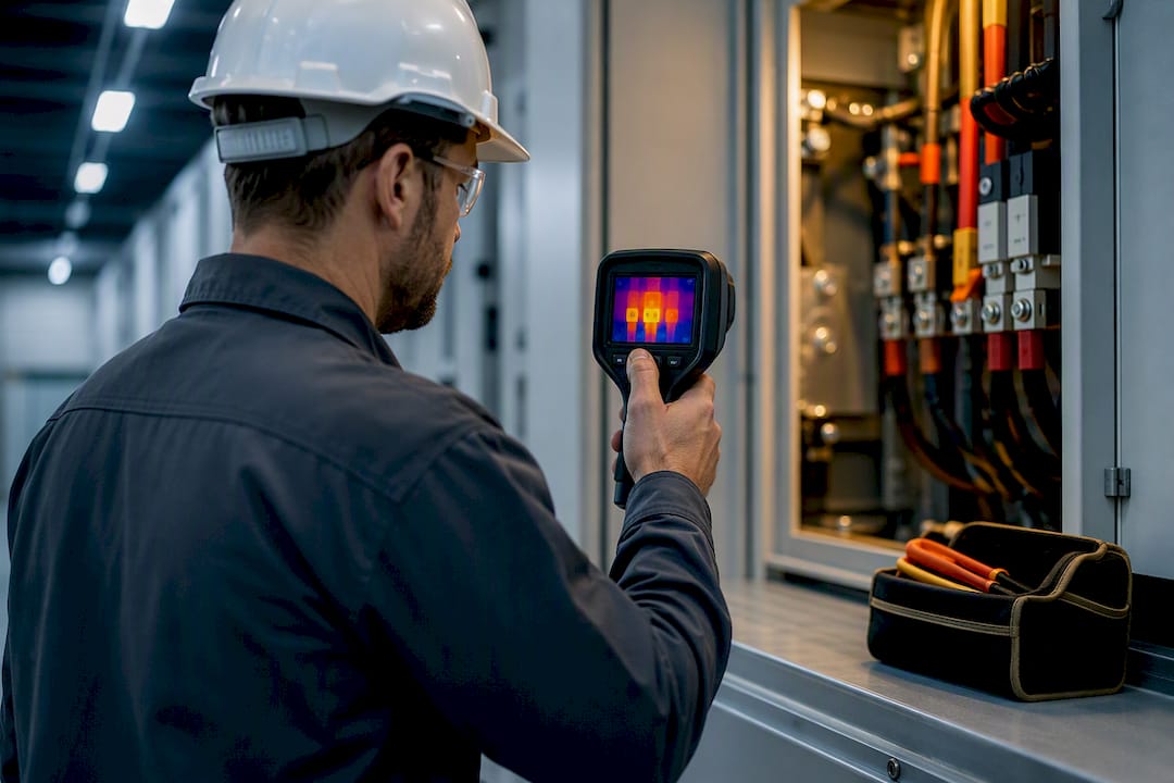
- Thermography for electrical panels, motor connections and insulation
- Oil analysis for gearboxes, hydraulics and compressors
- Ultrasound for bearing lubrication and leak detection
- Online sensor trending for continuous parameters like temperature and pressure
Sampling frequency has to match the shortest PF interval you expect from a given failure mode. Monthly vibration readings are worthless against a failure that develops in ten days. Match the technique’s resolution to the asset, not the other way round.
How do you build and measure a Curva PF from asset data?
Four data types feed a usable curve: failure logs with timestamps, inspection or sensor readings leading up to each failure, mean time between failures (MTBF), and mean time to repair (MTTR). Without failure logs tied to a timeline, you have no F point to measure back from.
Start by plotting condition readings against time for every recorded failure of a given mode, on the same asset class. Overlay several instances and the PF interval starts to emerge as a range rather than a single number. Building a practical PF workflow depends on this kind of historical rigour. Loose, undated inspection notes cannot be plotted against anything.
Survival-style indicators help here too. Tracking the proportion of assets still functioning at each time increment after a detected P gives you a distribution, not just an average, which matters when intervals vary widely between units.
Validation matters as much as the plot itself. Run repeatability checks: does the same detection technique flag the same failure mode consistently, or does it throw false positives that would send technicians chasing nothing? A curve built on noisy detection data will hand you PF intervals that are either dangerously optimistic or so conservative you inspect assets that never needed it. Recalibrate thresholds against real outcomes every few quarters.
Translating the PF interval into spares, labour and scheduling decisions
A PF interval is only useful once it drives a decision. Procurement lead time and specialist mobilisation time both need to fit comfortably inside the interval you have measured, with margin left for scheduling flexibility.
Three decision rules cover most situations:
- Schedule normally — the PF interval comfortably exceeds parts lead time and technician availability; slot the work into the next planned window.
- Act immediately — the interval is short relative to lead times, or the failure mode carries safety or production risk; treat detection as a work order trigger, not a diary entry.
- Continue monitoring — early-stage detection with a long interval and no immediate resource constraint; increase inspection frequency and reassess.
A gearbox oil analysis flags rising wear metal with an established six-week PF interval for that failure mode, and the replacement gearbox has a two-week lead time. That is a comfortable schedule decision, ideally timed against the next planned production stoppage. A thermography scan showing a hot connection on a critical motor circuit with a historically short interval, in contrast, belongs on today’s work order list regardless of how the production schedule looks.
Five practical steps to implement Curva PF in your maintenance programme
- Prepare data and KPIs. Pull failure logs, MTBF, MTTR and existing inspection records for the asset classes you want to start with.
- Select detection techniques and thresholds. Match vibration, thermography, oil analysis or sensor trending to the failure modes those assets actually experience, and set alert thresholds based on your historical data, not a generic manual figure.
- Define decision rules and work order triggers. Decide in advance which detected conditions schedule work, which trigger immediate action, and which simply increase monitoring frequency.
- Schedule and procure using PF lead times. Order parts and book technicians against the interval you have measured, aligned to production windows where possible. Fullyops’s essential preventive maintenance steps cover the scheduling mechanics in more depth.
- Verify outcomes and refine thresholds. Track whether interventions happened before F, whether emergency work orders dropped, and adjust thresholds every review cycle.
Common pitfalls, limitations and expert tips
The most common failure is applying one PF interval across an entire asset class regardless of operating context. A pump running continuous duty in a hot, dusty environment does not share a PF interval with the same model running intermittently in a clean plant room.
Detection without logistics is close to worthless: flagging a P three weeks early achieves nothing if the replacement part has a five-week lead time and nobody reserved it. Electrical assets carry a separate risk. Power factor correction work needs staged implementation and a harmonic study beforehand, since aggressive correction near variable-frequency drives can trigger resonance. Industry guidance generally targets a 0.90 to 0.95 power factor range and warns against pushing past roughly 0.97, where leading power factor becomes a new problem.
Consejo profesional: Recalibrate your PF thresholds every quarter using the last cycle’s actual outcomes, not just the manufacturer’s original spec sheet.
How a maintenance platform supports PF workflows
A CMMS built around work orders maps onto the PF process almost step for step. Sensor trend dashboards capture the P signal. Alert rules flag when a reading crosses a threshold. That alert can generate a work order automatically, reserve the required part from inventory, and assign it to the technician with the right specialism, all before anyone manually chases it down.
A detected bearing vibration trend on a conveyor motor triggers an alert, which raises a work order, reserves the replacement bearing from stock, and slots the job against the next maintenance window, closing with a verification report once complete. Fullyops is built around exactly this loop, and centralising detection data this way materially shortens the gap between spotting P and finishing the intervention. Fullyops’s work order management process shows how automated triggers reduce that lag in practice.
Impact of environmental and operational conditions on PF interval and curve shape
Two identical machines rarely share the same PF interval, because environment and duty cycle reshape the curve itself, not just its timing. Heat, humidity, dust and vibration from neighbouring equipment all accelerate the descent from P to F, often compressing an interval that looked comfortable on paper into something far tighter.
Loading pattern matters as much as ambient conditions. An asset running at a steady, moderate load tends to show a gradual, predictable decline, giving detection techniques a long, readable warning period. The same asset cycling between idle and peak load repeatedly develops fatigue-driven failure modes that can shorten the interval sharply and make the curve steeper near the end.
Maintenance history shapes the curve too. An asset with a track record of delayed lubrication or skipped inspections rarely follows the textbook curve shape; its PF interval shrinks because underlying condition was already compromised before the current monitoring cycle began.
This is why PF intervals should be treated as site specific rather than copied from a manufacturer’s baseline figure. A pump in a coastal, humid plant and the same model in a dry inland facility will show measurably different intervals for corrosion-driven failure modes. Practical programmes build rolling windows of local data and recalibrate as seasonal or process changes shift the operating envelope, rather than locking a single threshold in place indefinitely.
Relationship between Curva PF and RCM and predictive maintenance strategies
Reliability-centred maintenance (RCM) uses the PF curve as one of its core analytical tools when deciding which maintenance strategy fits a given failure mode. If a failure mode has a measurable, consistent PF interval and a detection technique exists that can catch it reliably, RCM logic points towards condition-based maintenance built on that curve. If no reliable detection method exists, or the interval is too short and unpredictable to act on, RCM typically defaults to fixed-interval preventive replacement or, for low-consequence failures, running to failure deliberately.
Predictive maintenance is essentially Curva PF thinking scaled up with continuous sensor data and statistical trending rather than periodic manual inspection. Where a technician might check vibration monthly with a handheld meter, a predictive system streams that data continuously and flags deviation from baseline automatically, catching P earlier and with more precision. Fullyops’s mantenimiento predictivo overview covers how continuous trending extends the PF interval you can actually act on.
The two approaches are not competing philosophies. RCM gives you the decision framework for which strategy suits which failure mode; predictive maintenance and condition monitoring give you the practical means to detect P early enough for that decision to matter. A maintenance programme that skips the RCM analysis and jumps straight to sensors on everything often ends up monitoring failure modes that never justified the investment, while a programme that does RCM analysis without investing in detection capability ends up with a strategy on paper it cannot actually execute.
How do you customise the PF curve for different equipment or industries?
No single PF interval works across a mixed fleet, and treating a rotating asset the same as a static one is one of the more common planning mistakes. Rotating equipment, bearings, gearboxes, pumps, typically gives the longest and most predictable intervals, because vibration and thermal signatures degrade gradually and detection techniques are mature. Electrical assets often show shorter, less linear intervals, particularly connection and insulation faults that can progress from barely detectable to catastrophic within days once moisture or thermal cycling accelerates degradation.
Structural and static components, tanks, pipework, structural steel, tend to have long PF intervals measured in months or years, detected through corrosion monitoring or periodic inspection rather than continuous sensors. Software-driven or electronic control systems sit at the opposite extreme: failure modes there are frequently binary, with almost no usable PF interval at all, which pushes the strategy towards redundancy rather than condition monitoring.
Industry context reshapes the same asset’s curve further. A motor in food processing faces washdown cycles and humidity that a similar motor in a dry warehouse never sees, shortening its effective PF interval for corrosion-related failure. A pump in a mining operation handling abrasive slurry wears through seals far faster than the same pump moving clean water.
Practical customisation starts by grouping assets into failure-mode families rather than by nameplate model, then building a separate curve for each family using its own failure history. Fullyops’s asset management resources cover how asset classification supports this kind of segmented approach at scale.
Integrating Curva PF data with a CMMS
Curva PF data earns its value the moment it stops living in a spreadsheet and starts triggering action inside your CMMS. The integration typically runs through three layers: detection data flowing in from sensors or inspection records, threshold logic that decides when a reading counts as P, and automated work order generation once that threshold trips.
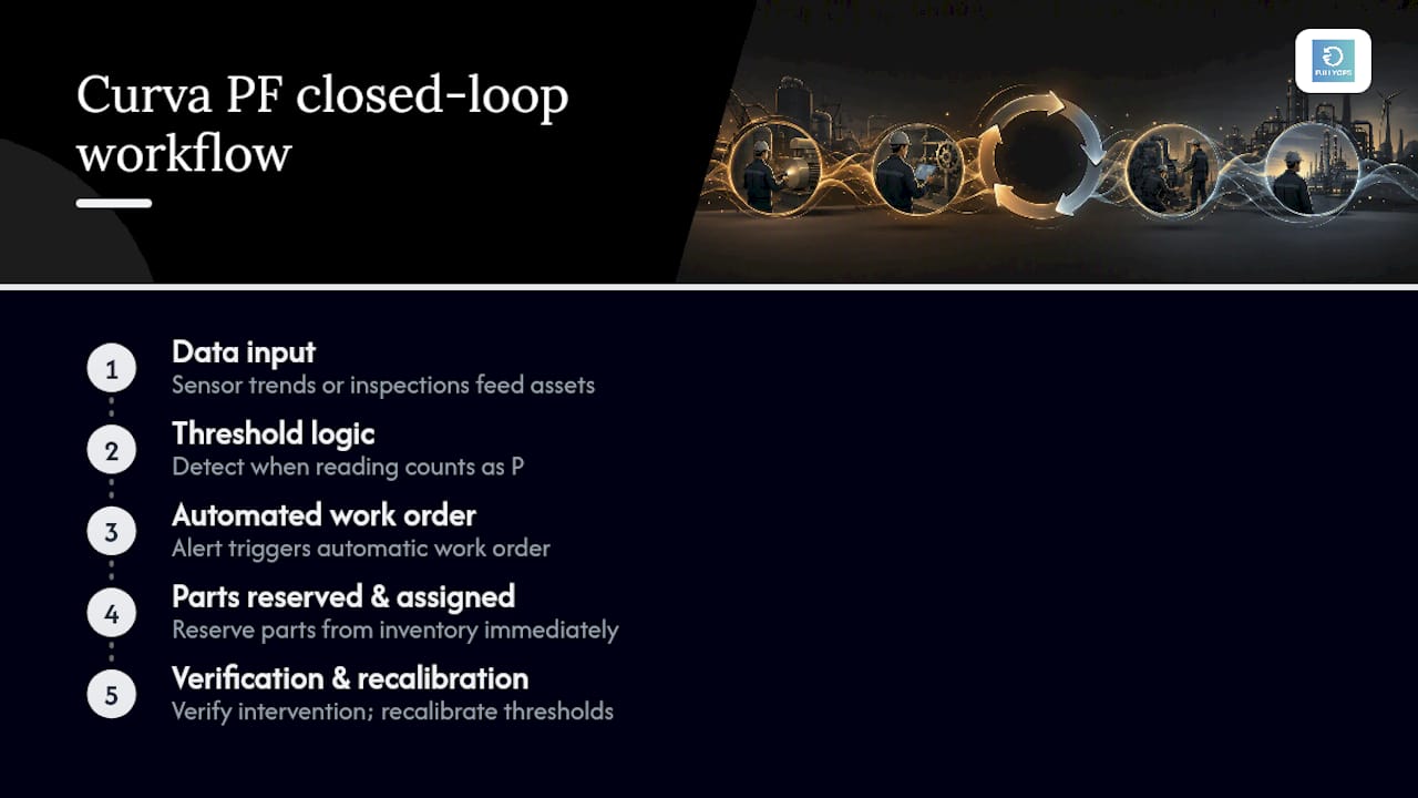
Practically, this means sensor trend data or manual inspection results feed directly into asset records rather than a separate log. When a reading crosses the defined threshold, the system raises an alert, and that alert can generate a work order automatically rather than waiting for someone to notice a flagged reading during a weekly review. Parts required for the likely intervention get reserved from inventory at the same moment, closing the gap between detection and mobilisation that undermines so many manual PF processes.
Reporting closes the loop. A CMMS with historical failure and intervention data lets you compare the PF interval you predicted against what actually happened, feeding directly back into threshold recalibration. Without that verification step, a PF programme drifts, because thresholds set once at the start never get tested against real outcomes.
Fullyops’s análisis de operaciones capability is built around exactly this closed loop, connecting detection, work orders, inventory and verification reporting so PF data does not stall at the alert stage.
Case studies showing successful application of Curva PF
A gearbox failure mode on a conveyor line offers the clearest illustration of PF logic paying off. Oil analysis consistently flags rising wear metal roughly six weeks before functional failure on that asset class. Once a maintenance team logs several of these events and confirms the interval, replacement gearboxes get ordered the moment wear metal crosses the threshold, timed to arrive during a planned production stoppage rather than an emergency shutdown.
A rotating equipment fleet with historically frequent emergency call-outs shows a similar pattern once vibration monitoring gets applied consistently across the same bearing type. Instead of waiting for audible failure, technicians start scheduling bearing replacement during the interval flagged by vibration trending, and the proportion of unplanned work orders for that failure mode drops as scheduled interventions replace emergency ones.
Electrical panels present a more cautionary example. Thermography catches a hot connection early enough to schedule a repair, but the PF interval for that specific fault type turns out to be short, days rather than weeks, because the underlying loose connection accelerates once resistive heating begins. Teams that treat every thermography flag with the same scheduling latitude as a slow-developing mechanical fault risk missing the window entirely; the lesson from cases like this is that interval length, not just detection, decides urgency.
Author perspective: why leaders should prioritise PF windows now
The maintenance managers who get the most from Curva PF are not the ones with the best sensors. They are the ones who fixed their logistics first. Detection means nothing if the part sits on backorder for six weeks against a four-week interval. Start small: pick one asset class, three to five similar machines, measure detection-to-action time and emergency work order rates before and after, and give it 90 days. That evidence sells the programme far better than any theoretical PF curve.
— Pedro
Consider Fullyops for PF-based maintenance workflows
Fullyops turns the PF interval from a spreadsheet exercise into a live workflow: detection alerts flow straight into work orders, spares get reserved automatically, and technicians see the job before the asset gets anywhere near functional failure. Where a manual process leaves detection and logistics disconnected, Fullyops closes that gap in one platform, which is exactly the failure point most PF programmes stumble on.
This article is published by Fullyops, and the platform is built to support the kind of PF-driven scheduling described above. If you manage a fleet where emergency work orders keep eating into planned maintenance time, book a look at field service management with Fullyops and see how a pilot on one asset class might run.
Sources
- Curva PF: o que é e como utilizá-la na manutenção – BibLus
- Power-factor correction – Wikipedia
- Understanding power factor – Enginist
PREGUNTAS FRECUENTES
What does P and F mean in a Curva PF?
P is potential failure, the earliest point deterioration becomes detectable, and F is functional failure, when the asset stops performing its intended function.
How long is a typical PF interval?
It varies enormously by failure mode and asset, from days for some electrical faults to months for gradual mechanical wear, which is why PF intervals should be measured from your own failure history rather than assumed.
Which detection method should I use first?
Match the method to the failure mode: vibration analysis for rotating equipment, thermography for electrical connections, oil analysis for gearboxes and hydraulics, and ultrasound for early bearing wear or leaks.
Can a CMMS automate the PF workflow?
Yes. A platform like Fullyops can turn a detection alert directly into a work order, reserve the required parts, and assign a technician, cutting the lag between spotting a potential failure and completing the fix.
What is the biggest mistake teams make with Curva PF?
Applying one generic interval across an entire asset class regardless of environment or duty cycle, and detecting P without having parts or technicians lined up to act within the window.